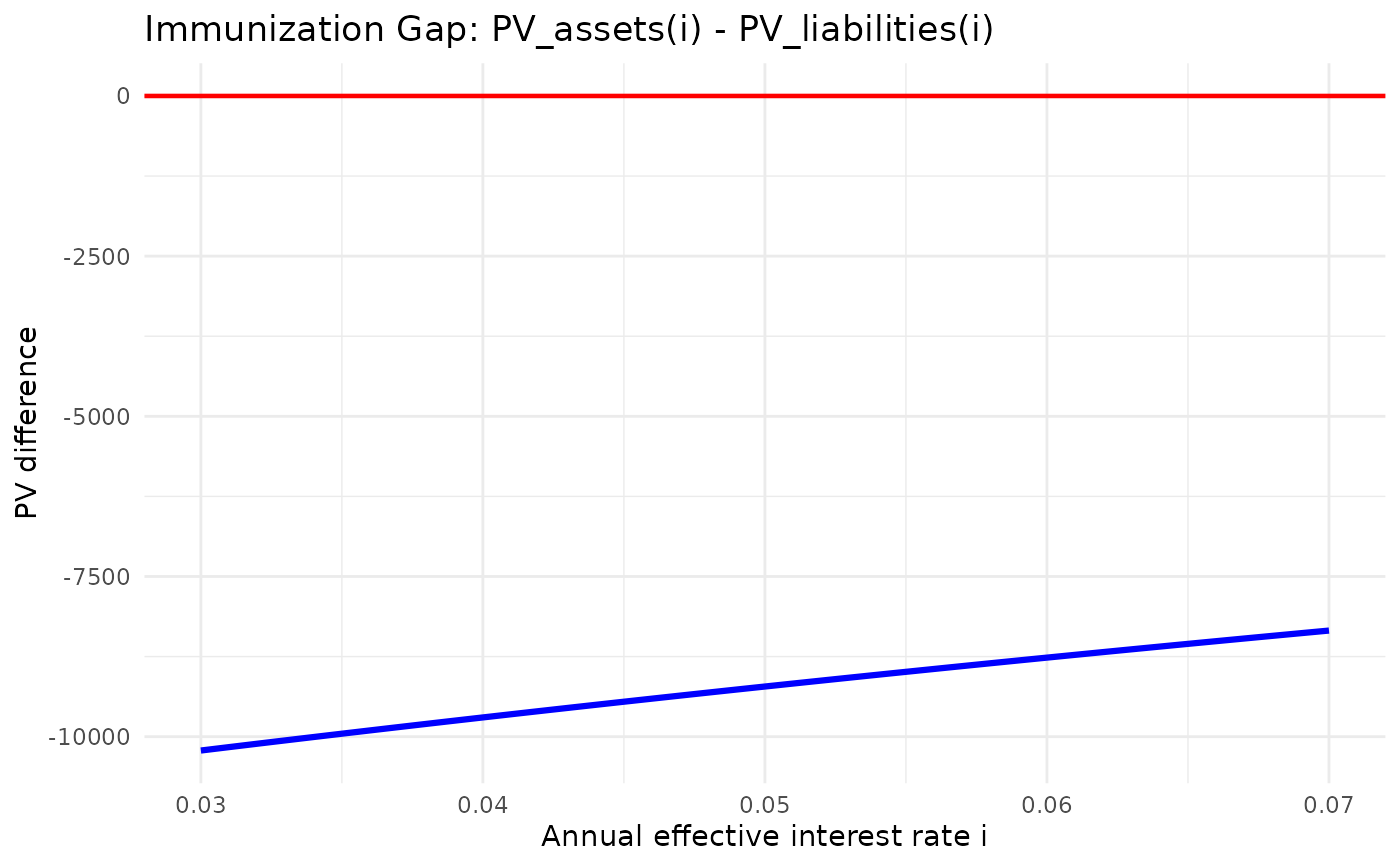
Plot immunization performance under interest-rate shifts

Computes and plots asset present value minus liability present value for an immunized portfolio under small interest rate changes. This allows visual evaluation of duration or duration-convexity immunization quality.

Usage

plot_immunization_gap(
  L,
  t,
  asset_cashflows,
  w,
  i,
  i_type = "effective",
  m = 1L,
  delta = 0.01,
  n_grid = 200L
)

Arguments

L

Numeric vector of liability payments.

t

Numeric vector of times of each liability payment.

asset_cashflows

A list where each element is a list with components $cf and $t, defining each asset's cash flow.

w

Numeric vector of portfolio weights or units. Must have the same length as asset_cashflows.

i

Base interest-rate input.

i_type

Character string indicating the interest-rate type. Allowed values are "effective", "nominal_interest", "nominal_discount", and "force".

m

Positive integer. Conversion frequency for nominal rates. Ignored for i_type = "effective" and i_type = "force".

delta

A numeric value defining the range of annual effective rates: from i_effective - delta to i_effective + delta, where i_effective is the annual effective rate equivalent to i, i_type, and m.

n_grid

Number of rate values to evaluate. Integer from 2 through .Machine$integer.max, with sufficient memory for the requested grid.

Value

A ggplot2 object showing the PV difference curve \(PV_A(i) - PV_L(i)\) and a zero reference line.

Details

This function follows the compact actuarial notation used throughout tidyactuarial: L denotes liabilities, t denotes payment times, w denotes asset weights, cf denotes cash flows, i denotes the interest-rate input, i_type denotes the interest-rate type, and m denotes the conversion frequency for nominal rates.

Let \(v(i) = 1/(1+i)\). For a liability stream \(L_k\) at time \(t_k\): $$PV_L(i) = \sum_k L_k \, v(i)^{t_k}$$

For a portfolio of assets with weights \(w_j\): $$PV_A(i) = \sum_j w_j \, PV_j(i)$$

The curve \(\Delta(i) = PV_A(i) - PV_L(i)\) illustrates immunization robustness. Under perfect duration immunization, this curve is tangent to zero at the base rate and non-negative nearby if the convexity condition is also met. The grid is expressed in annual effective yields and clipped, when needed, to the nearest representable value strictly above -1. Its base annual effective equivalent and grid endpoints must be finite and representable. Gap values combine signed weighted cash flows using log discounts, rather than subtracting separately overflowed portfolio values. Zero-weight assets contribute zero after validation. A nonfinite gap causes an explicit error. Recovery is limited by double precision and by cancellation already lost in input data; arbitrary extreme signed cancellation is not guaranteed. The graph reprices the supplied cash flows. Their consistency with the prices and sensitivities used to solve for weights remains the caller's responsibility. Matching convexity gives zero second derivative at the base yield and does not by itself ensure a positive surplus on either side.

See also

immunize_duration, immunize_duration_convexity, bond_duration, bond_convexity

Other immunization: immunize_duration(), immunize_duration_convexity()

Examples

# Two-asset duration immunization gap
plot_immunization_gap(
  L = c(5000, 8000),
  t = c(3, 7),
  asset_cashflows = list(
    list(cf = c(0, 0, 100), t = c(1, 2, 3)),
    list(cf = c(0, 0, 0, 0, 0, 0, 200), t = 1:7)
  ),
  w = c(5, 2.5),
  i = 0.05,
  delta = 0.02
)