Validate a yield curve and compute discount factors

Builds a tibble-first representation of a discrete yield curve and computes the corresponding spot discount factors, using compact actuarial notation.

Usage

yield_curve(
  .data = NULL,
  t = NULL,
  i = NULL,
  col_t = "t",
  col_i = "i",
  i_type = "effective",
  m = 1L,
  plot = FALSE,
  .out = "v",
  .out_plot = "yield_curve_plot",
  .keep = c("all", "used", "none"),
  .na = c("propagate", "error", "drop")
)

Arguments

.data: A data frame or tibble. If NULL, t and i must be supplied as numeric vectors.
t: Numeric vector of maturities in years when .data = NULL.
i: Numeric vector of spot-rate values when .data = NULL.
col_t: Name of the list-column containing maturities.
col_i: Name of the list-column containing spot rates.
i_type: Character vector indicating the spot-rate type. Allowed values are "effective", "nominal_interest", "nominal_discount", and "force". May have length 1 or the same length as each curve.
m: Positive integer vector giving the conversion frequency for nominal spot rates. May have length 1 or the same length as each curve.
plot: Logical. If TRUE, adds a list-column of ggplot2 objects.
.out: Name of the output list-column containing discount factors.
.out_plot: Name of the output list-column containing ggplot2 objects. Used only if plot = TRUE.
.keep: One of "all", "used", or "none".
.na: Missing-value handling policy: "propagate", "error", or "drop".

Value

A tibble. By default, it returns the original columns plus a new list-column named by .out containing discount-factor vectors. If plot = TRUE, it also adds a list-column named by .out_plot containing ggplot2 objects.

Details

Each row is treated as one curve. For tibble input, col_t and col_i must identify list-columns of equal-length numeric vectors. When .data = NULL, t and i must be numeric vectors and a one-row tibble is returned.

The discount factors are computed as: $$v_t = (1+i_t)^{-t}$$ where $i_t$ is the annual effective spot rate for maturity $t$.

If plot = TRUE, the function also returns a list-column of ggplot2 objects showing the spot yield curve for each row.

This function follows the compact actuarial notation used throughout tidyactuarial: t denotes maturity, i denotes the spot rate, i_type denotes the interest-rate type, and m denotes the conversion frequency for nominal spot rates.

Discount factors use the original log accumulation rate under the supplied convention. The reported annual effective equivalent may round to -1 or overflow to Inf while a finite discount factor remains recoverable. Final factors remain subject to double precision range. With .na = "propagate", an incomplete row keeps its position and has a NULL plot entry when plotting is requested.

References

Marcel B. Finan, A Basic Course in the Theory of Interest and Derivatives Markets: A Preparation for the Actuarial Exam FM/2, Section 53: The Term Structure of Interest Rates and Yield Curves.

Kellison, S. G. The Theory of Interest.

Examples

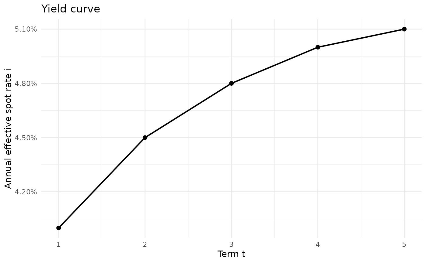
# Simple example
res <- yield_curve(
  t = c(1, 2, 3, 4, 5),
  i = c(0.040, 0.045, 0.048, 0.050, 0.051),
  plot = TRUE
)

res$yield_curve_plot[[1]]


# Multiple curves in a tibble
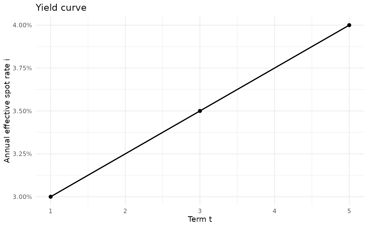
curves <- tibble::tibble(
  curve_id = c("A", "B"),
  t = list(c(1, 2, 3), c(1, 3, 5)),
  i = list(c(0.04, 0.05, 0.06), c(0.03, 0.035, 0.04))
)

res2 <- yield_curve(
  curves,
  col_t = "t",
  col_i = "i",
  plot = TRUE,
  .out = "v",
  .out_plot = "curve_plot"
)

res2$curve_plot[[2]]


# Nominal annual spot rates convertible semiannually
yield_curve(
  t = c(1, 2, 3),
  i = c(0.05, 0.055, 0.06),
  i_type = "nominal_interest",
  m = 2
)
#> # A tibble: 1 × 4
#>   t         i         v         i_effective
#>   <list>    <list>    <list>    <list>     
#> 1 <dbl [3]> <dbl [3]> <dbl [3]> <dbl [3]>