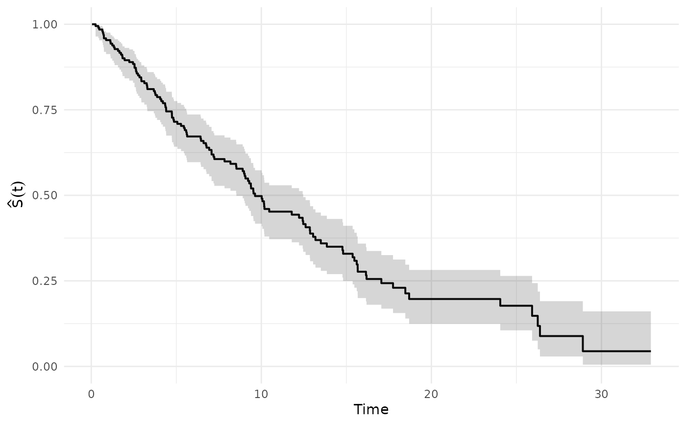
Kaplan–Meier survival curve and a lifetable-style life table
Source:R/km_lifetable.R
km_lifetable.RdFits the nonparametric Kaplan–Meier estimator \(\hat S(t)\) for
right-censored time-to-event data, computes Greenwood's variance estimator
for \(\hat S(t)\), and constructs a discrete life table by evaluating
\(\hat S(t)\) at user-provided cut points (breaks).
Usage
km_lifetable(
  time,
  status,
  entry = NULL,
  breaks = NULL,
  radix = 1e+05,
  conf_level = 0.95,
  assumption = c("UDD", "CF", "Balducci")
)
Arguments
- time
Numeric vector. Observed times (event or censoring times).
- status
Integer/numeric vector of the same length as
time. Use1for event (death),0for right-censoring.- entry
Optional numeric vector of entry times (left truncation / delayed entry). If provided, must have the same length as
timeand satisfyentry <= time. IfNULL, all individuals are assumed to enter at time 0.- breaks
Optional numeric vector of increasing cut points used to build the discrete life table (e.g.,
0:omega). IfNULL, defaults to integer ages from0toceiling(max(time)).- radix
Numeric. Life table radix used to scale \(\ell_x\) (default
1e5).- conf_level
Numeric in
(0,1). Confidence level for pointwise intervals for \(\hat S(t)\) computed via the log(-log) transformation (default0.95).- assumption
Character. Fractional-age assumption used to compute \(L_x\) within each interval:
"UDD","CF"(constant force), or"Balducci".
Value
A list with two tibbles:
km: tibble with columnstime,n_risk,d,censored,S,varS,seS,ci_low,ci_high.lifetable: tibble with columnsx,x_next,width,lx,dx,qx,px,mx,ax,Lx,Tx,ex. Carries class"lifetable"and standard attributes for compatibility with downstream functions.
Details
The resulting life table is intended for *experience-based* (empirical) life tables in actuarial/demographic contexts (e.g., cohort studies, population indicators). It is not a replacement for graduated/regulatory tables when smoothing, extrapolation, or product-specific selection effects are required.
**Kaplan–Meier estimator.** At each observed event time \(t_j\): $$\hat S(t) = \prod_{t_j \le t} \left(1 - \frac{d_j}{n_j}\right)$$ where \(n_j\) is the risk set size and \(d_j\) is the number of events. Greenwood's variance: $$\widehat{\mathrm{Var}}(\hat S(t)) = \hat S(t)^2 \sum_{t_j \le t} \frac{d_j}{n_j(n_j - d_j)}.$$ Pointwise confidence intervals use the log(-log) transformation.
**Life table mapping.** For each interval \([x, x + \Delta)\): $$\ell_x = \text{radix} \cdot \hat S(x), \quad d_x = \ell_x - \ell_{x+\Delta}, \quad q_x = d_x / \ell_x.$$
Exposure \(L_x = \int_x^{x+\Delta} \ell(t)\,dt\) is computed using the selected fractional-age assumption (Finan, Section 24):
UDD (Finan, Sec. 24.1): \(L_x \approx \tfrac{\ell_x + \ell_{x+\Delta}}{2} \Delta\)
CF (constant force, Finan, Sec. 24.2): \(L_x = \Delta \cdot (\ell_x - \ell_{x+\Delta}) / \ln(\ell_x / \ell_{x+\Delta})\)
Balducci (Finan, Sec. 24.3): \(L_x = \Delta \cdot \ell_x \ell_{x+\Delta} / (\ell_x - \ell_{x+\Delta}) \cdot \ln(\ell_x / \ell_{x+\Delta})\)
Additional columns follow Finan, Sections 23.3, 23.8–23.9:
\(T_x = \sum_{k \ge x} L_k\): total expected years lived after age \(x\) (Finan, Sec. 23.3).
\(\mathring{e}_x = T_x / \ell_x\): complete life expectancy (Finan, Sec. 23.3).
\(m_x = d_x / L_x\): central death rate (Finan, Sec. 23.9).
\(a_x = (L_x - \ell_{x+\Delta}\Delta) / d_x\): mean time lived within the interval by those who die, in years (not a fraction when interval width differs from one). Undefined if there are no deaths.
Nonfinite time/entry rows are omitted with a warning; the remaining sample
must be nonempty. Breaks are sorted and deduplicated. Beyond the last
observation, the KM step is held constant (no tail extrapolation is fitted).
CF/Balducci exposure at an interval ending at zero survival uses its zero
limit; positive deaths with zero exposure give infinite central mortality.
Confidence intervals remain undefined at survival zero or one.
Standard errors and intervals use Greenwood sums directly, preserving
small positive survival estimates without a fixed survival floor.
For delayed entry the risk set uses the existing inclusive convention
entry <= time; this is a deliberate convention at tied entries/events.
The lifetable component may have arbitrary interval widths: annual consumers
such as t_px require conversion to an annual grid with the needed
endpoint survivors; its class alone does not certify that conversion.
Examples
set.seed(1)
n <- 200
trueT <- rexp(n, rate = 0.08)
censT <- rexp(n, rate = 0.04)
time <- pmin(trueT, censT)
status <- as.integer(trueT <= censT)

out <- km_lifetable(time, status, breaks = 0:25, radix = 100000)
head(out$km)
#> # A tibble: 6 × 9
#>     time n_risk     d censored     S      varS     seS ci_low ci_high
#>    <dbl>  <dbl> <int>    <int> <dbl>     <dbl>   <dbl>  <dbl>   <dbl>
#> 1 0.0425    200     0        1 1     0         0       NA      NA
#> 2 0.0877    199     0        1 1     0         0       NA      NA
#> 3 0.113     198     0        1 1     0         0       NA      NA
#> 4 0.141     197     0        1 1     0         0       NA      NA
#> 5 0.191     196     0        1 1     0         0       NA      NA
#> 6 0.253     195     1        0 0.995 0.0000262 0.00512  0.964   0.999
head(out$lifetable)
#> # A tibble: 6 × 12
#>       x x_next width      lx    dx     qx    px     mx    ax     Lx     Tx    ex
#>   <int>  <int> <int>   <dbl> <dbl>  <dbl> <dbl>  <dbl> <dbl>  <dbl>  <dbl> <dbl>
#> 1     0      1     1 100000  4631. 0.0463 0.954 0.0474   0.5 97684. 1.16e6  11.6
#> 2     1      2     1  95369. 5872. 0.0616 0.938 0.0635   0.5 92433. 1.07e6  11.2
#> 3     2      3     1  89497. 6148. 0.0687 0.931 0.0711   0.5 86423. 9.74e5  10.9
#> 4     3      4     1  83349. 4636. 0.0556 0.944 0.0572   0.5 81031. 8.88e5  10.7
#> 5     4      5     1  78713. 7219. 0.0917 0.908 0.0961   0.5 75103. 8.07e5  10.3
#> 6     5      6     1  71494. 4294. 0.0601 0.940 0.0619   0.5 69347. 7.32e5  10.2

# Tidy pipeline: filter high-mortality intervals
out$lifetable |> dplyr::filter(qx > 0.05)
#> # A tibble: 18 × 12
#>        x x_next width     lx    dx     qx    px     mx    ax     Lx     Tx    ex
#>    <int>  <int> <int>  <dbl> <dbl>  <dbl> <dbl>  <dbl> <dbl>  <dbl>  <dbl> <dbl>
#>  1     1      2     1 95369. 5872. 0.0616 0.938 0.0635   0.5 92433. 1.07e6 11.2
#>  2     2      3     1 89497. 6148. 0.0687 0.931 0.0711   0.5 86423. 9.74e5 10.9
#>  3     3      4     1 83349. 4636. 0.0556 0.944 0.0572   0.5 81031. 8.88e5 10.7
#>  4     4      5     1 78713. 7219. 0.0917 0.908 0.0961   0.5 75103. 8.07e5 10.3
#>  5     5      6     1 71494. 4294. 0.0601 0.940 0.0619   0.5 69347. 7.32e5 10.2
#>  6     6      7     1 67200. 3935. 0.0586 0.941 0.0603   0.5 65232. 6.62e5  9.86
#>  7     7      8     1 63265. 3360. 0.0531 0.947 0.0546   0.5 61585. 5.97e5  9.44
#>  8     8      9     1 59905. 3558. 0.0594 0.941 0.0612   0.5 58126. 5.36e5  8.94
#>  9     9     10     1 56347. 6566. 0.117  0.883 0.124    0.5 53064. 4.77e5  8.47
#> 10    10     11     1 49781. 4551. 0.0914 0.909 0.0958   0.5 47505. 4.24e5  8.53
#> 11    12     13     1 44343. 5526. 0.125  0.875 0.133    0.5 41580. 3.32e5  7.49
#> 12    13     14     1 38817. 3837. 0.0988 0.901 0.104    0.5 36899. 2.91e5  7.48
#> 13    14     15     1 34980. 2058. 0.0588 0.941 0.0606   0.5 33951. 2.54e5  7.25
#> 14    15     16     1 32922. 5251. 0.159  0.841 0.173    0.5 30297. 2.20e5  6.67
#> 15    16     17     1 27672. 2129. 0.0769 0.923 0.0800   0.5 26608. 1.89e5  6.84
#> 16    17     18     1 25543. 2568. 0.101  0.899 0.106    0.5 24259. 1.63e5  6.37
#> 17    18     19     1 22975. 3282. 0.143  0.857 0.154    0.5 21334. 1.39e5  6.03
#> 18    24     25     1 19693. 1969. 0.1    0.9   0.105    0.5 18709. 1.87e4  0.95

# Compare UDD vs CF assumptions
udd <- km_lifetable(time, status, breaks = 0:20, assumption = "UDD")
cfm <- km_lifetable(time, status, breaks = 0:20, assumption = "CF")
c(ex_udd = udd$lifetable$ex[1], ex_cf = cfm$lifetable$ex[1])
#>   ex_udd    ex_cf
#> 10.66941 10.66335

# Plot the KM curve with plot_km
plot_km(out$km, time_col = "time", surv_col = "S",
        lower_col = "ci_low", upper_col = "ci_high")