Plot a Kaplan–Meier survival curve

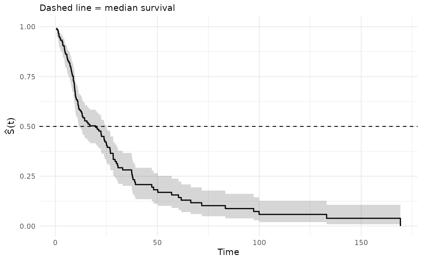
Creates a step-function plot of the Kaplan–Meier survival estimate \(\hat S(t)\) with optional pointwise confidence bands. Designed to work directly with the output of km_lifetable.

Usage

plot_km(
  km,
  time_col = "time",
  surv_col = "S",
  lower_col = "ci_low",
  upper_col = "ci_high",
  conf_int = TRUE,
  title = NULL
)

Arguments

km

A data frame or tibble with at least columns for time and survival. Can also be the full list returned by km_lifetable, in which case the $km component is extracted automatically.

time_col

Character. Name of the time column. Default "time".

surv_col

Character. Name of the survival column. Default "S" (matching km_lifetable output).

lower_col

Character. Name of the lower CI column. Default "ci_low" (matching km_lifetable output).

upper_col

Character. Name of the upper CI column. Default "ci_high" (matching km_lifetable output).

conf_int

Logical. If TRUE (default) and CI columns exist in km, plot a step-wise confidence ribbon.

title

Optional character string for the plot title.

Value

A ggplot object that can be further customised with additional ggplot2 layers.

Details

Both the survival curve and the confidence band are rendered as step functions (using geom_step), which is the correct representation for the KM estimator - a right-continuous step function that drops at each observed event time.

The confidence band uses geom_stepribbon logic: the data is internally expanded so that a ribbon-fill follows the step pattern rather than interpolating linearly between event times.

See also

km_lifetable for fitting the KM estimator and building the empirical life table.

Examples

set.seed(42)
n <- 150
time   <- rexp(n, rate = 0.05)
status <- rbinom(n, 1, prob = 0.7)

# Fit KM and plot directly
out <- km_lifetable(time, status, breaks = 0:30)

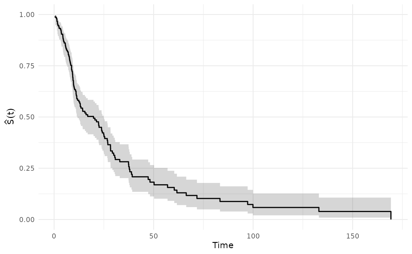
# Pass the full list - $km is extracted automatically
plot_km(out)


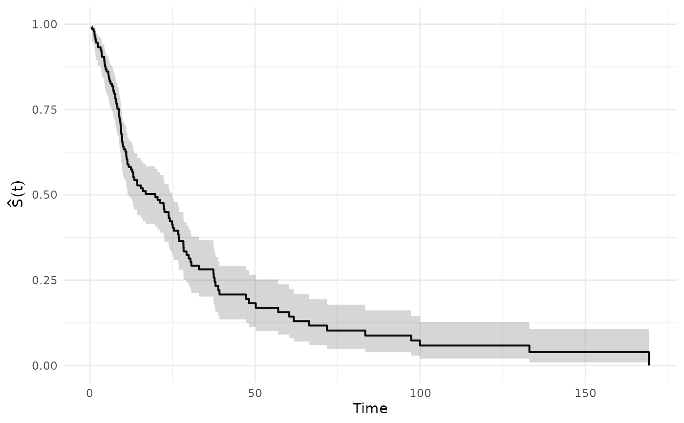# Or pass just the km tibble
plot_km(out$km)


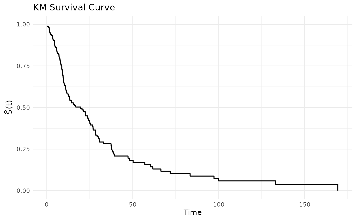
# Without confidence band
plot_km(out, conf_int = FALSE, title = "KM Survival Curve")


# Customise with ggplot2 layers
if (requireNamespace("ggplot2", quietly = TRUE)) {
  plot_km(out) +
    ggplot2::geom_hline(yintercept = 0.5, linetype = "dashed") +
    ggplot2::labs(subtitle = "Dashed line = median survival")
}