Plot discrete life-contingent cash flows

Separates contractual amounts, unconditional payment probabilities, expected cash flows and actuarial present-value contributions in editable panels. Consumes the payment-level output of apv_life_flow() without recomputing mortality, dates or interest, or an explicitly specified event table.

Usage

plot_contingent_cash_flow(
  .data,
  view = c("all", "contractual", "probability", "expected", "pv"),
  title = NULL,
  subtitle = NULL,
  x_label = NULL,
  show_labels = TRUE,
  label_size = 3.2,
  label_digits = 2L,
  label_format = c("auto", "full", "compact"),
  currency = "",
  col_inflow = "#1B9E77",
  col_outflow = "#D95F02",
  date_labels = "%Y-%m-%d"
)

Arguments

.data: A nonempty data frame or tibble. Supply an apv_life_flow() result, or columns t, cf, probability, discount and event. Optional date supplies the horizontal calendar axis. Optional expected_cf and pv are reused after consistency checks.
view: One of "all", "contractual", "probability", "expected", or "pv". The default shows four panels with separate vertical scales.
title, subtitle: Optional plot title and subtitle.
x_label: Optional horizontal axis label.
show_labels: Logical. Show amount/probability labels, omitting text that overlaps at rendering time. All payment rows remain in the plot.
label_size: Positive text size.
label_digits: Integer between 0 and 50 for monetary labels.
label_format: Monetary notation: "auto", "full", or "compact", as in plot_cash_flow(). Probabilities/weights use separate unitless labels.
currency: Monetary prefix; never applied to probabilities or weights.
col_inflow, col_outflow: Colors for positive and negative monetary flows.
date_labels: Calendar label format for ggplot2::scale_x_date().

Value

An editable ggplot2 object. Its tibble data has one row per payment per selected measure: row, t, x, event, measure, value, plot_value and label. value retains original units; extreme monetary panels use scaled plot_value with the power of ten in the panel title.

Details

For a binary payment event $E_j$, contractual signed amount $C_j$, payment date $t_j$ and deterministic discount $d_j$, the panels show $$C_j,\quad p_j=P(E_j),\quad C_jp_j,\quad C_jp_jd_j.$$ Probabilities are unconditional relative to the common initial actuarial state, not conditional annual mortality rates. For survival payments, $p_j={}_{t_j}p_x$. For death in $(a,b]$, $p_j={}_ap_x-{}_bp_x={}_ap_x\,{}_{b-a}q_{x+a}$. A benefit payable at the end of that interval is discounted to its payment date, not the exact time of death. Continuous death-time benefits require a different model.

In explicit event tables, event contains "survival", "death_interval" or "certain" (the last requires probability one). Interval probabilities must be supplied; the plot never differences arbitrary rows of a stream. Rows may represent different events at the same date; probabilities are never added or netted. Coincident stems can overlap; points identify their endpoints and no payment date is moved. Negative amounts denote outflows.

For new apv_life_flow() results, contingency metadata distinguishes binary survival from a reversionary expected benefit fraction. For the latter, surv_prob is $P(\text{all alive})+\alpha P(\text{some but not all alive})$, not generally a probability: the second panel is labeled Expected benefit fraction. Results lacking metadata use the conservative label Payment weight; no event is inferred from column names alone. Explicit tables can use event = "weighted" for such finite multipliers as well.

life_contract() stores a specification, and insurance_x()/annuity_x() return aggregate values rather than payment schedules. These objects cannot be plotted directly: supply an explicit payment table instead. The plot does not expand contracts or reevaluate actuarial assumptions.

All required numeric values must be finite, with nonnegative t and discount, and probabilities in $[0,1]$ for binary events. Missing or inconsistent rows are rejected, never silently removed. Supplied expected amounts and PVs must agree with the identities to relative tolerance 1e-10; they are retained, not replaced. The plot ignores cached APV/cumulative attributes and sums the displayed contributions. Calendar dates and stored t are retained; in particular apv_life_flow() uses actual days/365.25. All rows must share a valuation origin and monetary unit.

Examples

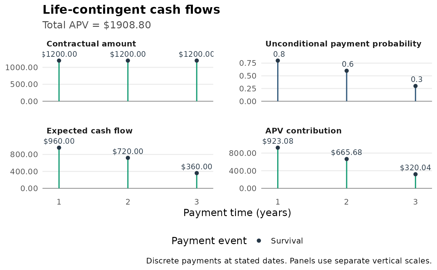
lt <- tibble::tibble(x = 60:64, lx = c(1000, 800, 600, 300, 0))
apv_life_flow(lt, ages = 60, t = 1:3, cf = rep(1200, 3), i = 0.04) |>
  plot_contingent_cash_flow(currency = "$")


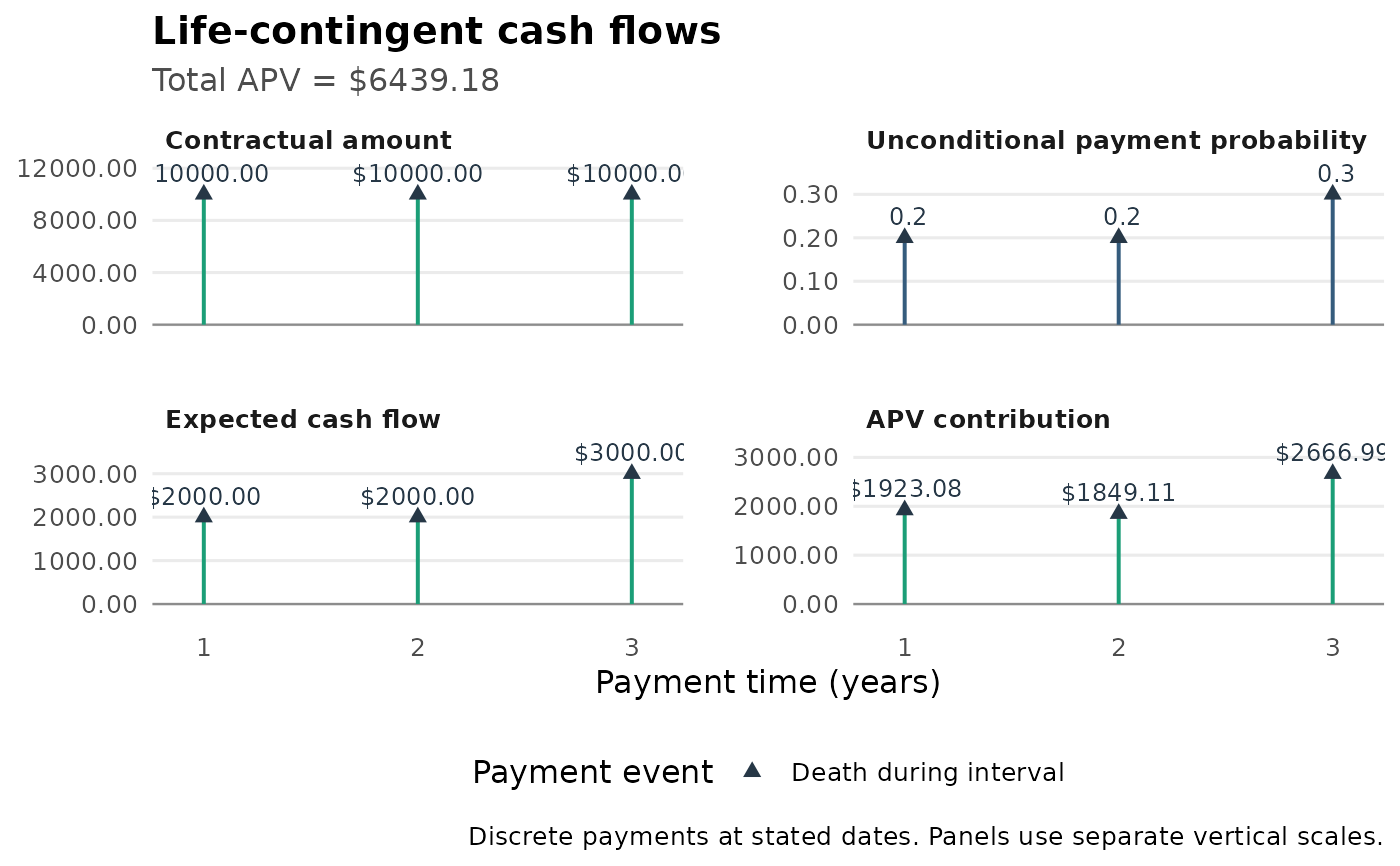
# Three-year term insurance, paid at each year-end of death.
# P(j-1 < T <= j) = (l[x+j-1] - l[x+j]) / l[x], not q[x+j-1].
death_flows <- tibble::tibble(
  t = 1:3, cf = rep(10000, 3),
  probability = c(200, 200, 300) / 1000,
  discount = 1.04^-(1:3), event = "death_interval"
)
death_flows |> plot_contingent_cash_flow(currency = "$")

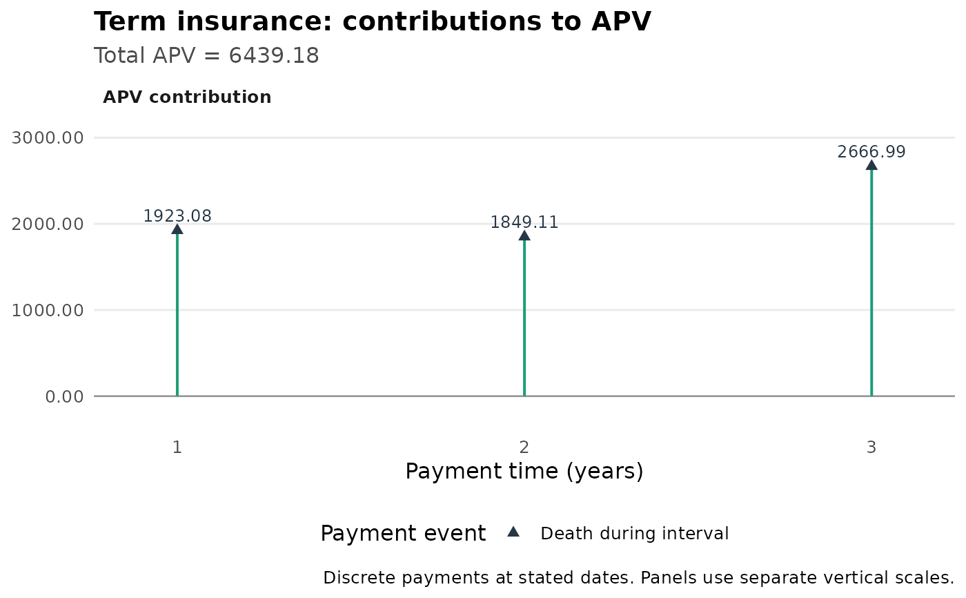
death_flows |> plot_contingent_cash_flow(view = "pv") +
  ggplot2::labs(title = "Term insurance: contributions to APV")

Usage

Arguments

Value

Details

See also

Examples